Chapter 4. Building Good Training Sets – Data Preprocessing

The quality of the data and the amount of useful information that it contains are key factors that determine how well a machine learning algorithm can learn. Therefore, it is absolutely critical that we make sure to examine and preprocess a dataset before we feed it to a learning algorithm. In this chapter, we will discuss the essential data preprocessing techniques that will help us to build good machine learning models.

The topics that we will cover in this chapter are as follows:

• Removing and imputing missing values from the dataset
• Getting categorical data into shape for machine learning algorithms
• Selecting relevant features for the model construction

Dealing with missing data

It is not uncommon in real-world applications that our samples are missing one or more values for various reasons. There could have been an error in the data collection process, certain measurements are not applicable, particular fields could have been simply left blank in a survey, for example. We typically see missing values as the blank spaces in our data table or as placeholder strings such as NaN (Not A Number).

Unfortunately, most computational tools are unable to handle such missing values or would produce unpredictable results if we simply ignored them. Therefore, it is crucial that we take care of those missing values before we proceed with further analyses. But before we discuss several techniques for dealing with missing values, let's create a simple example data frame from a CSV (comma-separated values) file to get a better grasp of the problem:

>>> import pandas as pd
>>> from io import StringIO
>>> csv_data = '''A,B,C,D
... 1.0,2.0,3.0,4.0
... 5.0,6.0,,8.0
... 0.0,11.0,12.0,'''
>>> # If you are using Python 2.7, you need
>>> # to convert the string to unicode:
>>> # csv_data = unicode(csv_data)
>>> df = pd.read_csv(StringIO(csv_data))
>>> df
   A   B   C   D
0  1   2   3   4
1  5   6 NaN   8
2  0  11  12 NaN

Using the preceding code, we read CSV-formatted data into a pandas DataFrame via the read_csv function and noticed that the two missing cells were replaced by NaN. The StringIO function in the preceding code example was simply used for the purposes of illustration. It allows us to read the string assigned to csv_data into a pandas DataFrame as if it was a regular CSV file on our hard drive.

For a larger DataFrame, it can be tedious to look for missing values manually; in this case, we can use the isnull method to return a DataFrame with Boolean values that indicate whether a cell contains a numeric value (False) or if data is missing (True). Using the sum method, we can then return the number of missing values per column as follows:

>>> df.isnull().sum()
A    0
B    0
C    1
D    1
dtype: int64

This way, we can count the number of missing values per column; in the following subsections, we will take a look at different strategies for how to deal with this missing data.

Note

Although scikit-learn was developed for working with NumPy arrays, it can sometimes be more convenient to preprocess data using pandas' DataFrame. We can always access the underlying NumPy array of the DataFrame via the values attribute before we feed it into a scikit-learn estimator:

>>> df.values
array([[  1.,   2.,   3.,   4.],
       [  5.,   6.,  nan,   8.],
       [ 10.,  11.,  12.,  nan]])

Eliminating samples or features with missing values

One of the easiest ways to deal with missing data is to simply remove the corresponding features (columns) or samples (rows) from the dataset entirely; rows with missing values can be easily dropped via the dropna method:

>>> df.dropna()
   A  B  C  D
0  1  2  3  4

Similarly, we can drop columns that have at least one NaN in any row by setting the axis argument to 1:

>>> df.dropna(axis=1)
   A   B
0  1   2
1  5   6
2  0  11

The dropna method supports several additional parameters that can come in handy:

# only drop rows where all columns are NaN
>>> df.dropna(how='all')  

# drop rows that have not at least 4 non-NaN values
>>> df.dropna(thresh=4)  

# only drop rows where NaN appear in specific columns (here: 'C')
>>> df.dropna(subset=['C'])

Although the removal of missing data seems to be a convenient approach, it also comes with certain disadvantages; for example, we may end up removing too many samples, which will make a reliable analysis impossible. Or, if we remove too many feature columns, we will run the risk of losing valuable information that our classifier needs to discriminate between classes. In the next section, we will thus look at one of the most commonly used alternatives for dealing with missing values: interpolation techniques.

Imputing missing values

Often, the removal of samples or dropping of entire feature columns is simply not feasible, because we might lose too much valuable data. In this case, we can use different interpolation techniques to estimate the missing values from the other training samples in our dataset. One of the most common interpolation techniques is mean imputation, where we simply replace the missing value by the mean value of the entire feature column. A convenient way to achieve this is by using the Imputer class from scikit-learn, as shown in the following code:

>>> from sklearn.preprocessing import Imputer
>>> imr = Imputer(missing_values='NaN', strategy='mean', axis=0)
>>> imr = imr.fit(df)
>>> imputed_data = imr.transform(df.values)
>>> imputed_data
array([[  1.,   2.,   3.,   4.],
       [  5.,   6.,   3.,   8.],
       [ 10.,  11.,  12.,   4.]])

Here, we replaced each NaN value by the corresponding mean, which is separately calculated for each feature column. If we changed the setting axis=0 to axis=1, we'd calculate the row means. Other options for the strategy parameter are median or most_frequent, where the latter replaces the missing values by the most frequent values. This is useful for imputing categorical feature values.

Understanding the scikit-learn estimator API

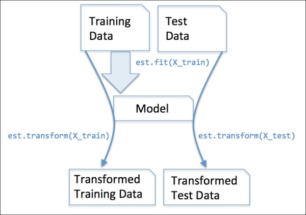
In the previous section, we used the Imputer class from scikit-learn to impute missing values in our dataset. The Imputer class belongs to the so-called transformer classes in scikit-learn that are used for data transformation. The two essential methods of those estimators are fit and transform. The fit method is used to learn the parameters from the training data, and the transform method uses those parameters to transform the data. Any data array that is to be transformed needs to have the same number of features as the data array that was used to fit the model. The following figure illustrates how a transformer fitted on the training data is used to transform a training dataset as well as a new test dataset:

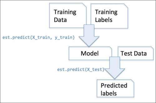
The classifiers that we used in Chapter 3, A Tour of Machine Learning Classifiers Using Scikit-Learn, belong to the so-called estimators in scikit-learn with an API that is conceptually very similar to the transformer class. Estimators have a predict method but can also have a transform method, as we will see later. As you may recall, we also used the fit method to learn the parameters of a model when we trained those estimators for classification. However, in supervised learning tasks, we additionally provide the class labels for fitting the model, which can then be used to make predictions about new data samples via the predict method, as illustrated in the following figure:

Handling categorical data

So far, we have only been working with numerical values. However, it is not uncommon that real-world datasets contain one or more categorical feature columns. When we are talking about categorical data, we have to further distinguish between nominal and ordinal features. Ordinal features can be understood as categorical values that can be sorted or ordered. For example, T-shirt size would be an ordinal feature, because we can define an order XL > L > M. In contrast, nominal features don't imply any order and, to continue with the previous example, we could think of T-shirt color as a nominal feature since it typically doesn't make sense to say that, for example, red is larger than blue.

Before we explore different techniques to handle such categorical data, let's create a new data frame to illustrate the problem:

>>> import pandas as pd
>>> df = pd.DataFrame([
...            ['green', 'M', 10.1, 'class1'], 
...            ['red', 'L', 13.5, 'class2'], 
...            ['blue', 'XL', 15.3, 'class1']])
>>> df.columns = ['color', 'size', 'price', 'classlabel']
>>> df
   color size  price classlabel
0  green    M   10.1     class1
1    red    L   13.5     class2
2   blue   XL   15.3     class1

As we can see in the preceding output, the newly created DataFrame contains a nominal feature (color), an ordinal feature (size), and a numerical feature (price) column. The class labels (assuming that we created a dataset for a supervised learning task) are stored in the last column. The learning algorithms for classification that we discuss in this book do not use ordinal information in class labels.

Mapping ordinal features

To make sure that the learning algorithm interprets the ordinal features correctly, we need to convert the categorical string values into integers. Unfortunately, there is no convenient function that can automatically derive the correct order of the labels of our size feature. Thus, we have to define the mapping manually. In the following simple example, let's assume that we know the difference between features, for example, .

>>> size_mapping = {
...                 'XL': 3,
...                 'L': 2,
...                 'M': 1}
>>> df['size'] = df['size'].map(size_mapping)
>>> df
   color  size  price classlabel
0  green     1   10.1     class1
1    red     2   13.5     class2
2   blue     3   15.3     class1

If we want to transform the integer values back to the original string representation at a later stage, we can simply define a reverse-mapping dictionary inv_size_mapping = {v: k for k, v in size_mapping.items()} that can then be used via the pandas' map method on the transformed feature column similar to the size_mapping dictionary that we used previously.

Encoding class labels

Many machine learning libraries require that class labels are encoded as integer values. Although most estimators for classification in scikit-learn convert class labels to integers internally, it is considered good practice to provide class labels as integer arrays to avoid technical glitches. To encode the class labels, we can use an approach similar to the mapping of ordinal features discussed previously. We need to remember that class labels are not ordinal, and it doesn't matter which integer number we assign to a particular string-label. Thus, we can simply enumerate the class labels starting at 0:

>>> import numpy as np
>>> class_mapping = {label:idx for idx,label in
...                  enumerate(np.unique(df['classlabel']))}
>>> class_mapping
{'class1': 0, 'class2': 1}

Next we can use the mapping dictionary to transform the class labels into integers:

>>> df['classlabel'] = df['classlabel'].map(class_mapping)
>>> df
   color  size  price  classlabel
0  green     1   10.1           0
1    red     2   13.5           1
2   blue     3   15.3           0

We can reverse the key-value pairs in the mapping dictionary as follows to map the converted class labels back to the original string representation:

>>> inv_class_mapping = {v: k for k, v in class_mapping.items()}
>>> df['classlabel'] = df['classlabel'].map(inv_class_mapping)
>>> df
   color  size  price classlabel
0  green     1   10.1     class1
1    red     2   13.5     class2
2   blue     3   15.3     class1

Alternatively, there is a convenient LabelEncoder class directly implemented in scikit-learn to achieve the same:

>>> from sklearn.preprocessing import LabelEncoder
>>> class_le = LabelEncoder()
>>> y = class_le.fit_transform(df['classlabel'].values)
>>> y
array([0, 1, 0])

Note that the fit_transform method is just a shortcut for calling fit and transform separately, and we can use the inverse_transform method to transform the integer class labels back into their original string representation:

>>> class_le.inverse_transform(y)
array(['class1', 'class2', 'class1'], dtype=object)

Performing one-hot encoding on nominal features

In the previous section, we used a simple dictionary-mapping approach to convert the ordinal size feature into integers. Since scikit-learn's estimators treat class labels without any order, we used the convenient LabelEncoder class to encode the string labels into integers. It may appear that we could use a similar approach to transform the nominal color column of our dataset, as follows:

>>> X = df[['color', 'size', 'price']].values
>>> color_le = LabelEncoder()
>>> X[:, 0] = color_le.fit_transform(X[:, 0])
>>> X
array([[1, 1, 10.1],
       [2, 2, 13.5],
       [0, 3, 15.3]], dtype=object)

After executing the preceding code, the first column of the NumPy array X now holds the new color values, which are encoded as follows:

• blue → 0
• green → 1
• red → 2

If we stop at this point and feed the array to our classifier, we will make one of the most common mistakes in dealing with categorical data. Can you spot the problem? Although the color values don't come in any particular order, a learning algorithm will now assume that green is larger than blue, and red is larger than green. Although this assumption is incorrect, the algorithm could still produce useful results. However, those results would not be optimal.

A common workaround for this problem is to use a technique called one-hot encoding. The idea behind this approach is to create a new dummy feature for each unique value in the nominal feature column. Here, we would convert the color feature into three new features: blue, green, and red. Binary values can then be used to indicate the particular color of a sample; for example, a blue sample can be encoded as blue=1, green=0, red=0. To perform this transformation, we can use the OneHotEncoder that is implemented in the scikit-learn.preprocessing module:

>>> from sklearn.preprocessing import OneHotEncoder
>>> ohe = OneHotEncoder(categorical_features=[0])
>>> ohe.fit_transform(X).toarray()
array([[  0. ,   1. ,   0. ,   1. ,  10.1],
       [  0. ,   0. ,   1. ,   2. ,  13.5],
       [  1. ,   0. ,   0. ,   3. ,  15.3]])

When we initialized the OneHotEncoder, we defined the column position of the variable that we want to transform via the categorical_features parameter (note that color is the first column in the feature matrix X). By default, the OneHotEncoder returns a sparse matrix when we use the transform method, and we converted the sparse matrix representation into a regular (dense) NumPy array for the purposes of visualization via the toarray method. Sparse matrices are simply a more efficient way of storing large datasets, and one that is supported by many scikit-learn functions, which is especially useful if it contains a lot of zeros. To omit the toarray step, we could initialize the encoder as OneHotEncoder(…,sparse=False) to return a regular NumPy array.

An even more convenient way to create those dummy features via one-hot encoding is to use the get_dummies method implemented in pandas. Applied on a DataFrame, the get_dummies method will only convert string columns and leave all other columns unchanged:

>>> pd.get_dummies(df[['price', 'color', 'size']])
   price  size  color_blue  color_green  color_red
0   10.1     1           0            1          0
1   13.5     2           0            0          1
2   15.3     3           1            0          0