Partitioning a dataset in training and test sets

We briefly introduced the concept of partitioning a dataset into separate datasets for training and testing in Wine dataset. After we have preprocessed the dataset, we will explore different techniques for feature selection to reduce the dimensionality of a dataset.

The Wine dataset is another open-source dataset that is available from the UCI machine learning repository (https://archive.ics.uci.edu/ml/datasets/Wine); it consists of 178 wine samples with 13 features describing their different chemical properties.

Using the pandas library, we will directly read in the open source Wine dataset from the UCI machine learning repository:

>>> df_wine = pd.read_csv('https://archive.ics.uci.edu/ml/machine-learning-databases/wine/wine.data', header=None)
>>> df_wine.columns = ['Class label', 'Alcohol', 
...                    'Malic acid', 'Ash', 
...                    'Alcalinity of ash', 'Magnesium', 
...                    'Total phenols', 'Flavanoids',
...                    'Nonflavanoid phenols', 
...                    'Proanthocyanins', 
...                    'Color intensity', 'Hue', 
...                    'OD280/OD315 of diluted wines', 
...                    'Proline']
>>>  print('Class labels', np.unique(df_wine['Class label']))
Class labels [1 2 3]
>>> df_wine.head()

The 13 different features in the Wine dataset, describing the chemical properties of the 178 wine samples, are listed in the following table:

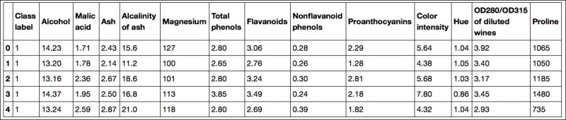
The samples belong to one of three different classes, 1, 2, and 3, which refer to the three different types of grapes that have been grown in different regions in Italy.

A convenient way to randomly partition this dataset into a separate test and training dataset is to use the train_test_split function from scikit-learn's cross_validation submodule:

>>> from sklearn.cross_validation import train_test_split
>>> X, y = df_wine.iloc[:, 1:].values, df_wine.iloc[:, 0].values
>>> X_train, X_test, y_train, y_test = \
...        train_test_split(X, y, test_size=0.3, random_state=0)

First, we assigned the NumPy array representation of feature columns 1-13 to the variable X, and we assigned the class labels from the first column to the variable y. Then, we used the train_test_split function to randomly split X and y into separate training and test datasets. By setting test_size=0.3 we assigned 30 percent of the wine samples to X_test and y_test, and the remaining 70 percent of the samples were assigned to X_train and y_train, respectively.

Note

If we are dividing a dataset into training and test datasets, we have to keep in mind that we are withholding valuable information that the learning algorithm could benefit from. Thus, we don't want to allocate too much information to the test set. However, the smaller the test set, the more inaccurate the estimation of the generalization error. Dividing a dataset into training and test sets is all about balancing this trade-off. In practice, the most commonly used splits are 60:40, 70:30, or 80:20, depending on the size of the initial dataset. However, for large datasets, 90:10 or 99:1 splits into training and test subsets are also common and appropriate. Instead of discarding the allocated test data after model training and evaluation, it is a good idea to retrain a classifier on the entire dataset for optimal performance.

Bringing features onto the same scale

Feature scaling is a crucial step in our preprocessing pipeline that can easily be forgotten. Decision trees and random forests are one of the very few machine learning algorithms where we don't need to worry about feature scaling. However, the majority of machine learning and optimization algorithms behave much better if features are on the same scale, as we saw in gradient descent optimization algorithm.

The importance of feature scaling can be illustrated by a simple example. Let's assume that we have two features where one feature is measured on a scale from 1 to 10 and the second feature is measured on a scale from 1 to 100,000. When we think of the squared error function in Adaline in with a Euclidean distance measure; the computed distances between samples will be dominated by the second feature axis.

Now, there are two common approaches to bringing different features onto the same scale: normalization and standardization. Those terms are often used quite loosely in different fields, and the meaning has to be derived from the context. Most often, normalization refers to the rescaling of the features to a range of [0, 1], which is a special case of min-max scaling. To normalize our data, we can simply apply the min-max scaling to each feature column, where the new value of a sample can be calculated as follows:

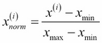
Here, is a particular sample, is the smallest value in a feature column, and the largest value, respectively.

The min-max scaling procedure is implemented in scikit-learn and can be used as follows:

>>> from sklearn.preprocessing import MinMaxScaler
>>> mms = MinMaxScaler()
>>> X_train_norm = mms.fit_transform(X_train)
>>> X_test_norm = mms.transform(X_test)

Although normalization via min-max scaling is a commonly used technique that is useful when we need values in a bounded interval, standardization can be more practical for many machine learning algorithms. The reason is that many linear models, such as the logistic regression and SVM that we remember from standardization, we center the feature columns at mean 0 with standard deviation 1 so that the feature columns take the form of a normal distribution, which makes it easier to learn the weights. Furthermore, standardization maintains useful information about outliers and makes the algorithm less sensitive to them in contrast to min-max scaling, which scales the data to a limited range of values.

The procedure of standardization can be expressed by the following equation:

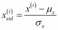
Here, is the sample mean of a particular feature column and the corresponding standard deviation, respectively.

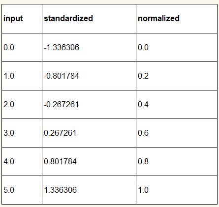
The following table illustrates the difference between the two commonly used feature scaling techniques, standardization and normalization on a simple sample dataset consisting of numbers 0 to 5:

Similar to MinMaxScaler, scikit-learn also implements a class for standardization:

>>> from sklearn.preprocessing import StandardScaler
>>> stdsc = StandardScaler()
>>> X_train_std = stdsc.fit_transform(X_train)
>>> X_test_std = stdsc.transform(X_test)

Again, it is also important to highlight that we fit the StandardScaler only once on the training data and use those parameters to transform the test set or any new data point.

Selecting meaningful features

If we notice that a model performs much better on a training dataset than on the test dataset, this observation is a strong indicator for overfitting. Overfitting means that model fits the parameters too closely to the particular observations in the training dataset but does not generalize well to real data—we say that the model has a high variance. A reason for overfitting is that our model is too complex for the given training data and common solutions to reduce the generalization error are listed as follows:

• Collect more training data
• Introduce a penalty for complexity via regularization
• Choose a simpler model with fewer parameters
• Reduce the dimensionality of the data

Collecting more training data is often not applicable. In the next chapter, we will learn about a useful technique to check whether more training data is helpful at all. In the following sections and subsections, we will look at common ways to reduce overfitting by regularization and dimensionality reduction via feature selection.

Sparse solutions with L1 regularization

We recall from L2 regularization is one approach to reduce the complexity of a model by penalizing large individual weights, where we defined the L2 norm of our weight vector w as follows:

Another approach to reduce the model complexity is the related L1 regularization:

Here, we simply replaced the square of the weights by the sum of the absolute values of the weights. In contrast to L2 regularization, L1 regularization yields sparse feature vectors; most feature weights will be zero. Sparsity can be useful in practice if we have a high-dimensional dataset with many features that are irrelevant, especially cases where we have more irrelevant dimensions than samples. In this sense, L1 regularization can be understood as a technique for feature selection.

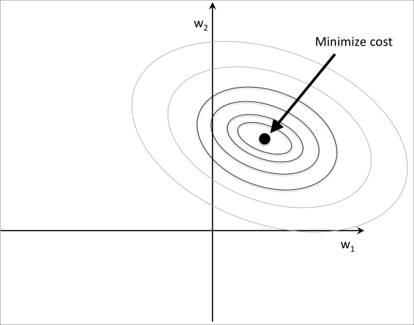
To better understand how L1 regularization encourages sparsity, let's take a step back and take a look at a geometrical interpretation of regularization. Let's plot the contours of a convex cost function for two weight coefficients and . Here, we will consider the sum of the squared errors (SSE) cost function that we used for Adaline in Chapter 2, Training Machine Learning Algorithms for Classification, since it is symmetrical and easier to draw than the cost function of logistic regression; however, the same concepts apply to the latter. Remember that our goal is to find the combination of weight coefficients that minimize the cost function for the training data, as shown in the following figure (the point in the middle of the ellipses):

Now, we can think of regularization as adding a penalty term to the cost function to encourage smaller weights; or, in other words, we penalize large weights.

Thus, by increasing the regularization strength via the regularization parameter , we shrink the weights towards zero and decrease the dependence of our model on the training data. Let's illustrate this concept in the following figure for the L2 penalty term.

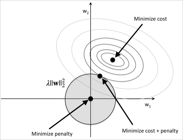
The quadratic L2 regularization term is represented by the shaded ball. Here, our weight coefficients cannot exceed our regularization budget—the combination of the weight coefficients cannot fall outside the shaded area. On the other hand, we still want to minimize the cost function. Under the penalty constraint, our best effort is to choose the point where the L2 ball intersects with the contours of the unpenalized cost function. The larger the value of the regularization parameter gets, the faster the penalized cost function grows, which leads to a narrower L2 ball. For example, if we increase the regularization parameter towards infinity, the weight coefficients will become effectively zero, denoted by the center of the L2 ball. To summarize the main message of the example: our goal is to minimize the sum of the unpenalized cost function plus the penalty term, which can be understood as adding bias and preferring a simpler model to reduce the variance in the absence of sufficient training data to fit the model.

Now let's discuss L1 regularization and sparsity. The main concept behind L1 regularization is similar to what we have discussed here. However, since the L1 penalty is the sum of the absolute weight coefficients (remember that the L2 term is quadratic), we can represent it as a diamond shape budget, as shown in the following figure:

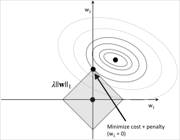
In the preceding figure, we can see that the contour of the cost function touches the L1 diamond at . Since the contours of an L1 regularized system are sharp, it is more likely that the optimum—that is, the intersection between the ellipses of the cost function and the boundary of the L1 diamond—is located on the axes, which encourages sparsity. The mathematical details of why L1 regularization can lead to sparse solutions are beyond the scope of this book. If you are interested, an excellent section on L2 versus L1 regularization can be found in section 3.4 of The Elements of Statistical Learning, Trevor Hastie, Robert Tibshirani, and Jerome Friedman, Springer.

For regularized models in scikit-learn that support L1 regularization, we can simply set the penalty parameter to 'l1' to yield the sparse solution:

>>> from sklearn.linear_model import LogisticRegression
>>> LogisticRegression(penalty='l1')

Applied to the standardized Wine data, the L1 regularized logistic regression would yield the following sparse solution:

>>> lr = LogisticRegression(penalty='l1', C=0.1)
>>> lr.fit(X_train_std, y_train)
>>> print('Training accuracy:', lr.score(X_train_std, y_train))
Training accuracy: 0.983870967742
>>> print('Test accuracy:', lr.score(X_test_std, y_test))
Test accuracy: 0.981481481481

Both training and test accuracies (both 98 percent) do not indicate any overfitting of our model. When we access the intercept terms via the lr.intercept_ attribute, we can see that the array returns three values:

>>> lr.intercept_
array([-0.38379237, -0.1580855 , -0.70047966])

Since we the fit the LogisticRegression object on a multiclass dataset, it uses the One-vs-Rest (OvR) approach by default where the first intercept belongs to the model that fits class 1 versus class 2 and 3; the second value is the intercept of the model that fits class 2 versus class 1 and 3; and the third value is the intercept of the model that fits class 3 versus class 1 and 2, respectively:

>>> lr.coef_
array([[ 0.280, 0.000, 0.000, -0.0282, 0.000,
         0.000, 0.710, 0.000, 0.000, 0.000,
         0.000, 0.000, 1.236],
       [-0.644, -0.0688 , -0.0572, 0.000, 0.000,
         0.000, 0.000, 0.000, 0.000, -0.927,
         0.060, 0.000, -0.371],
       [ 0.000, 0.061, 0.000, 0.000, 0.000,
         0.000, -0.637, 0.000, 0.000, 0.499,
        -0.358, -0.570, 0.000
       ]])

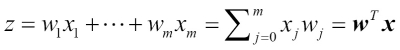
The weight array that we accessed via the lr.coef_ attribute contains three rows of weight coefficients, one weight vector for each class. Each row consists of 13 weights where each weight is multiplied by the respective feature in the 13-dimensional Wine dataset to calculate the net input:

We notice that the weight vectors are sparse, which means that they only have a few non-zero entries. As a result of the L1 regularization, which serves as a method for feature selection, we just trained a model that is robust to the potentially irrelevant features in this dataset.

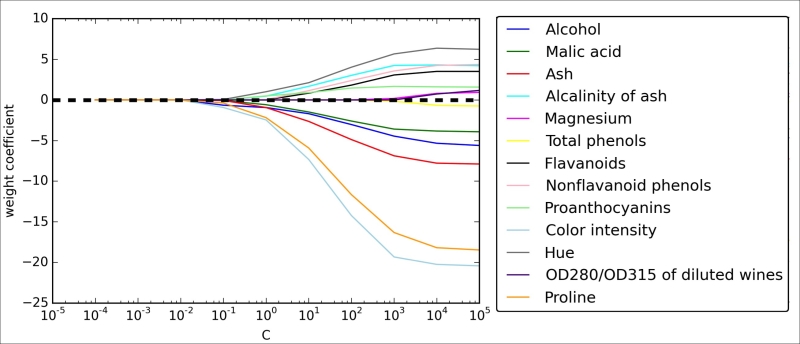
Lastly, let's plot the regularization path, which is the weight coefficients of the different features for different regularization strengths:

>>> import matplotlib.pyplot as plt
>>> fig = plt.figure()
>>> ax = plt.subplot(111)   
>>> colors = ['blue', 'green', 'red', 'cyan', 
...          'magenta', 'yellow', 'black', 
...          'pink', 'lightgreen', 'lightblue', 
...          'gray', 'indigo', 'orange']
>>> weights, params = [], []
>>> for c in np.arange(-4, 6):
...     lr = LogisticRegression(penalty='l1', 
...                             C=10**c, 
...                             random_state=0)
...     lr.fit(X_train_std, y_train)
...     weights.append(lr.coef_[1])
...     params.append(10**c)
>>> weights = np.array(weights)
>>> for column, color in zip(range(weights.shape[1]), colors):
...     plt.plot(params, weights[:, column],
...              label=df_wine.columns[column+1],
...              color=color)
>>> plt.axhline(0, color='black', linestyle='--', linewidth=3)
>>> plt.xlim([10**(-5), 10**5])
>>> plt.ylabel('weight coefficient')
>>> plt.xlabel('C')
>>> plt.xscale('log')
>>> plt.legend(loc='upper left')
>>> ax.legend(loc='upper center', 
...           bbox_to_anchor=(1.38, 1.03),
...           ncol=1, fancybox=True)
>>> plt.show()

The resulting plot provides us with further insights about the behavior of L1 regularization. As we can see, all features weights will be zero if we penalize the model with a strong regularization parameter (); is the inverse of the regularization parameter .

Sequential feature selection algorithms

An alternative way to reduce the complexity of the model and avoid overfitting is dimensionality reduction via feature selection, which is especially useful for unregularized models. There are two main categories of dimensionality reduction techniques: feature selection and feature extraction. Using feature selection, we select a subset of the original features. In feature extraction, we derive information from the feature set to construct a new feature subspace. In this section, we will take a look at a classic family of feature selection algorithms. In the next chapter, Chapter 5, Compressing Data via Dimensionality Reduction, we will learn about different feature extraction techniques to compress a dataset onto a lower dimensional feature subspace.

Sequential feature selection algorithms are a family of greedy search algorithms that are used to reduce an initial d-dimensional feature space to a k-dimensional feature subspace where k < d. The motivation behind feature selection algorithms is to automatically select a subset of features that are most relevant to the problem to improve computational efficiency or reduce the generalization error of the model by removing irrelevant features or noise, which can be useful for algorithms that don't support regularization. A classic sequential feature selection algorithm is Sequential Backward Selection (SBS), which aims to reduce the dimensionality of the initial feature subspace with a minimum decay in performance of the classifier to improve upon computational efficiency. In certain cases, SBS can even improve the predictive power of the model if a model suffers from overfitting.

Note

Greedy algorithms make locally optimal choices at each stage of a combinatorial search problem and generally yield a suboptimal solution to the problem in contrast to exhaustive search algorithms, which evaluate all possible combinations and are guaranteed to find the optimal solution. However, in practice, an exhaustive search is often computationally not feasible, whereas greedy algorithms allow for a less complex, computationally more efficient solution.

The idea behind the SBS algorithm is quite simple: SBS sequentially removes features from the full feature subset until the new feature subspace contains the desired number of features. In order to determine which feature is to be removed at each stage, we need to define criterion function that we want to minimize. The criterion calculated by the criterion function can simply be the difference in performance of the classifier after and before the removal of a particular feature. Then the feature to be removed at each stage can simply be defined as the feature that maximizes this criterion; or, in more intuitive terms, at each stage we eliminate the feature that causes the least performance loss after removal. Based on the preceding definition of SBS, we can outline the algorithm in 4 simple steps:

1. Initialize the algorithm with , where d is the dimensionality of the full feature space .
2. Determine the feature that maximizes the criterion ) where .
3. Remove the feature from the feature set: – 1 = .
4. Terminate if k equals the number of desired features, if not, go to step 2.

   Note

   You can find a detailed evaluation of several sequential feature algorithms in Comparative Study of Techniques for Large Scale Feature Selection, F. Ferri, P. Pudil, M. Hatef, and J. Kittler. Comparative study of techniques for large-scale feature selection. Pattern Recognition in Practice IV, pages 403–413, 1994.

Unfortunately, the SBS algorithm is not implemented in scikit-learn, yet. But since it is so simple, let's go ahead and implement it in Python from scratch:

from sklearn.base import clone
from itertools import combinations
import numpy as np
from sklearn.cross_validation import train_test_split
from sklearn.metrics import accuracy_score

class SBS():
    def __init__(self, estimator, k_features, 
        scoring=accuracy_score,
        test_size=0.25, random_state=1):
        self.scoring = scoring
        self.estimator = clone(estimator)
        self.k_features = k_features
        self.test_size = test_size
        self.random_state = random_state

    def fit(self, X, y):
        X_train, X_test, y_train, y_test = \
                train_test_split(X, y, test_size=self.test_size, 
                                 random_state=self.random_state)

        dim = X_train.shape[1]
        self.indices_ = tuple(range(dim))
        self.subsets_ = [self.indices_]
        score = self._calc_score(X_train, y_train, 
                                 X_test, y_test, self.indices_)
        self.scores_ = [score]

        while dim > self.k_features:
            scores = []
            subsets = []

            for p in combinations(self.indices_, r=dim-1):
                score = self._calc_score(X_train, y_train, 
                                         X_test, y_test, p)
                scores.append(score)
                subsets.append(p)

            best = np.argmax(scores)
            self.indices_ = subsets[best]
            self.subsets_.append(self.indices_)
            dim -= 1

            self.scores_.append(scores[best])
        self.k_score_ = self.scores_[-1]

        return self

    def transform(self, X):
        return X[:, self.indices_]

    def _calc_score(self, X_train, y_train, 
                          X_test, y_test, indices):
        self.estimator.fit(X_train[:, indices], y_train)
        y_pred = self.estimator.predict(X_test[:, indices])
        score = self.scoring(y_test, y_pred)
        return score

In the preceding implementation, we defined the k_features parameter to specify the desired number of features we want to return. By default, we use the accuracy_score from scikit-learn to evaluate the performance of a model and estimator for classification on the feature subsets. Inside the while loop of the fit method, the feature subsets created by the itertools.combination function are evaluated and reduced until the feature subset has the desired dimensionality. In each iteration, the accuracy score of the best subset is collected in a list self.scores_ based on the internally created test dataset X_test. We will use those scores later to evaluate the results. The column indices of the final feature subset are assigned to self.indices_, which we can use via the transform method to return a new data array with the selected feature columns. Note that, instead of calculating the criterion explicitly inside the fit method, we simply removed the feature that is not contained in the best performing feature subset.

Now, let's see our SBS implementation in action using the KNN classifier from scikit-learn:

>>> from sklearn.neighbors import KNeighborsClassifier
>>> import matplotlib.pyplot as plt
>>> knn = KNeighborsClassifier(n_neighbors=2)
>>> sbs = SBS(knn, k_features=1)
>>> sbs.fit(X_train_std, y_train)

Although our SBS implementation already splits the dataset into a test and training dataset inside the fit function, we still fed the training dataset X_train to the algorithm. The SBS fit method will then create new training-subsets for testing (validation) and training, which is why this test set is also called validation dataset. This approach is necessary to prevent our original test set becoming part of the training data.

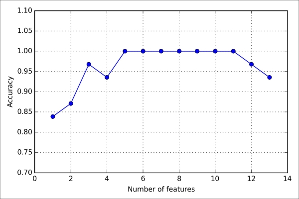
Remember that our SBS algorithm collects the scores of the best feature subset at each stage, so let's move on to the more exciting part of our implementation and plot the classification accuracy of the KNN classifier that was calculated on the validation dataset. The code is as follows:

>>> k_feat = [len(k) for k in sbs.subsets_]
>>> plt.plot(k_feat, sbs.scores_, marker='o')
>>> plt.ylim([0.7, 1.1])
>>> plt.ylabel('Accuracy')
>>> plt.xlabel('Number of features')
>>> plt.grid()
>>> plt.show()

As we can see in the following plot, the accuracy of the KNN classifier improved on the validation dataset as we reduced the number of features, which is likely due to a decrease of the curse of dimensionality that we discussed in the context of the KNN algorithm in Chapter 3, A Tour of Machine Learning Classifiers Using Scikit-learn. Also, we can see in the following plot that the classifier achieved 100 percent accuracy for k={5, 6, 7, 8, 9, 10}:

To satisfy our own curiosity, let's see what those five features are that yielded such a good performance on the validation dataset:

>>> k5 = list(sbs.subsets_[8])
>>> print(df_wine.columns[1:][k5])
Index(['Alcohol', 'Malic acid', 'Alcalinity of ash', 'Hue', 'Proline'], dtype='object')

Using the preceding code, we obtained the column indices of the 5-feature subset from the 9th position in the sbs.subsets_ attribute and returned the corresponding feature names from the column-index of the pandas Wine DataFrame.

Next let's evaluate the performance of the KNN classifier on the original test set:

>>> knn.fit(X_train_std, y_train)
>>> print('Training accuracy:', knn.score(X_train_std, y_train))
Training accuracy: 0.983870967742
>>> print('Test accuracy:', knn.score(X_test_std, y_test))
Test accuracy: 0.944444444444

In the preceding code, we used the complete feature set and obtained ~98.4 percent accuracy on the training dataset. However, the accuracy on the test dataset was slightly lower (~94.4 percent), which is an indicator of a slight degree of overfitting. Now let's use the selected 5-feature subset and see how well KNN performs:

>>> knn.fit(X_train_std[:, k5], y_train)
>>> print('Training accuracy:', 
...        knn.score(X_train_std[:, k5], y_train))
Training accuracy: 0.959677419355
>>> print('Test accuracy:',
...        knn.score(X_test_std[:, k5], y_test))
Test accuracy: 0.962962962963

Using fewer than half of the original features in the Wine dataset, the prediction accuracy on the test set improved by almost 2 percent. Also, we reduced overfitting, which we can tell from the small gap between test (~96.3 percent) and training (~96.0 percent) accuracy.

Note

Feature selection algorithms in scikit-learn

There are many more feature selection algorithms available via scikit-learn. Those include recursive backward elimination based on feature weights, tree-based methods to select features by importance, and univariate statistical tests. A comprehensive discussion of the different feature selection methods is beyond the scope of this book, but a good summary with illustrative examples can be found at http://scikit-learn.org/stable/modules/feature_selection.html.

Assessing feature importance with random forests

In the previous sections, you learned how to use L1 regularization to zero out irrelevant features via logistic regression and use the SBS algorithm for feature selection. Another useful approach to select relevant features from a dataset is to use a random forest, an ensemble technique that we introduced in Chapter 3, A Tour of Machine Learning Classifiers Using Scikit-learn. Using a random forest, we can measure feature importance as the averaged impurity decrease computed from all decision trees in the forest without making any assumptions whether our data is linearly separable or not. Conveniently, the random forest implementation in scikit-learn already collects feature importances for us so that we can access them via the feature_importances_ attribute after fitting a RandomForestClassifier. By executing the following code, we will now train a forest of 10,000 trees on the Wine dataset and rank the 13 features by their respective importance measures. Remember (from our discussion in Chapter 3, A Tour of Machine Learning Classifiers Using Scikit-learn) that we don't need to use standardized or normalized tree-based models. The code is as follows:

>>> from sklearn.ensemble import RandomForestClassifier
>>> feat_labels = df_wine.columns[1:]
>>> forest = RandomForestClassifier(n_estimators=10000,
...                                random_state=0,
...                                n_jobs=-1)
>>> forest.fit(X_train, y_train)
>>> importances = forest.feature_importances_
>>> indices = np.argsort(importances)[::-1]
>>> for f in range(X_train.shape[1]):
...     print("%2d) %-*s %f" % (f + 1, 30, 
...                             feat_labels[f], 
...                             importances[indices[f]]))
1) Alcohol                        0.182508
2) Malic acid                     0.158574
3) Ash                            0.150954
4) Alcalinity of ash              0.131983
5) Magnesium                      0.106564
6) Total phenols                  0.078249
7) Flavanoids                     0.060717
8) Nonflavanoid phenols           0.032039
9) Proanthocyanins                0.025385
10) Color intensity               0.022369
11) Hue                           0.022070
12) OD280/OD315 of diluted wines  0.014655
13) Proline                       0.013933
>>> plt.title('Feature Importances')
>>> plt.bar(range(X_train.shape[1]), 
...         importances[indices],
...         color='lightblue', 
...         align='center')
>>> plt.xticks(range(X_train.shape[1]), 
...            feat_labels, rotation=90)
>>> plt.xlim([-1, X_train.shape[1]])
>>> plt.tight_layout()
>>> plt.show()

After executing the preceding code, we created a plot that ranks the different features in the Wine dataset by their relative importance; note that the feature importances are normalized so that they sum up to 1.0.

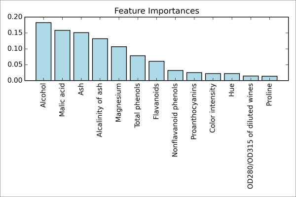
We can conclude that the alcohol content of wine is the most discriminative feature in the dataset based on the average impurity decrease in the 10,000 decision trees. Interestingly, the three top-ranked features in the preceding plot are also among the top five features in the selection by the SBS algorithm that we implemented in the previous section. However, as far as interpretability is concerned, the random forest technique comes with an important gotcha that is worth mentioning. For instance, if two or more features are highly correlated, one feature may be ranked very highly while the information of the other feature(s) may not be fully captured. On the other hand, we don't need to be concerned about this problem if we are merely interested in the predictive performance of a model rather than the interpretation of feature importances. To conclude this section about feature importances and random forests, it is worth mentioning that scikit-learn also implements a transform method that selects features based on a user-specified threshold after model fitting, which is useful if we want to use the RandomForestClassifier as a feature selector and intermediate step in a scikit-learn pipeline, which allows us to connect different preprocessing steps with an estimator, as we will see in Chapter 6, Learning Best Practices for Model Evaluation and Hyperparameter Tuning. For example, we could set the threshold to 0.15 to reduce the dataset to the 3 most important features, Alcohol, Malic acid, and Ash using the following code:

>>> X_selected = forest.transform(X_train, threshold=0.15)
>>> X_selected.shape
(124, 3)

Summary

We started this chapter by looking at useful techniques to make sure that we handle missing data correctly. Before we feed data to a machine learning algorithm, we also have to make sure that we encode categorical variables correctly, and we have seen how we can map ordinal and nominal features values to integer representations.

Moreover, we briefly discussed L1 regularization, which can help us to avoid overfitting by reducing the complexity of a model. As an alternative approach for removing irrelevant features, we used a sequential feature selection algorithm to select meaningful features from a dataset.

In the next chapter, you will learn about yet another useful approach to dimensionality reduction: feature extraction. It allows us to compress features onto a lower dimensional subspace rather than removing features entirely as in feature selection.