- R Programming By Example
- Omar Trejo Navarro
- 501字
- 2021-07-02 21:30:45
Checking no collinearity with correlations
To check no collinearity, we could use a number of different techniques. For example, for those familiar with linear algebra, the condition number is a measure of how singular a matrix is, where singularity would imply perfect collinearity among the covariates. This number could provide a measure of this collinearity. Another technique is to use the Variance Inflation Factor, which is a more formal technique that provides a measure of how much a regression's variance is increased because of collinearity. Another, and a more common, way of checking this is with simple correlations. Are any variables strongly correlated among themselves in the sense that there could be a direct relation among them? If so, then we may have a multicollinearity problem. To get a sense of how correlated our variables are, we will use the correlations matrix techniques shown in Chapter 2, Understanding Votes with Descriptive Statistics.
The following code shows how correlations work in R:
library(corrplot)
corrplot(corr = cor(data[, numerical_variables]), tl.col = "black", tl.cex = 0.6)
As you can see, the strong correlations (either positive or negative) are occurring intra-groups not inter-groups, meaning that variables that measure the same thing in different ways appear to be highly correlated, while variables that measure different things don't appear to be highly correlated.
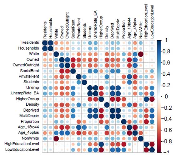
For example, Age_18to44 and Age_45plus are variables that measure age, and we expect them to have a negative relation since the higher the percentage of young people in a ward is, by necessity, the percentage of older people is lower. The same relation can be seen in the housing group (Owned, OwnedOutright, SocialRent, and PrivateRent), the employment group (Unemp, UnempRate_EA, and HigherOccup), the deprived group (Deprived and MultiDepriv), ethnic group (White and NonWhite), the residency group (Residents and Households), and the education group (LowEducationLevel and HighEducationLevel). If you pick variables belonging to different groups, the number of strong correlations is significantly lower, but it's there. For example, HigherOccup is strongly correlated to HighEducationLevel and LowEducationLevel, positively and negatively, respectively. Also, variables in the housing group seem to be correlated with variables in the age group. These kinds of relations are expected and natural since highly educated people will most probably have better jobs, and young people probably can't afford a house yet, so they rent. As analysts, we can assume that these variables are in fact measuring different aspects of society and continue on with our analysis. However, these are still things you may want to keep in mind when interpreting the results, and we may also want to only include one of the variables in each group to avoid inter-group collinearity, but we'll avoid these complexities and continue with our analysis for now.
Linear regression is one of those types of models that require criteria from the analyst to be accepted or rejected. In our specific case, it seems that our model's assumptions are valid enough and we may safely use it to provide credible predictions as we will do in the following sections.