Three constraints on computing performance – CPU, RAM, and disk I/O

First, let's see how R programs are executed in a computer. This is a very simplified version of what actually happens, but it suffices for us to understand the performance limitations of R. The following figure illustrates the steps required to execute an R program.

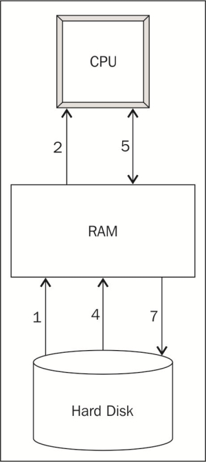
Steps to execute an R program

Take for example, this simple R program, which loads some data from a CSV file, computes the column sums, and writes the results into another CSV file:

data <- read.csv("mydata.csv")
totals <- colSums(data)
write.csv(totals, "totals.csv")

We use the numbering to understand the preceding diagram:

From this depiction of the computing process, we can see a few places where performance bottlenecks can occur:

Sometimes, you might encounter these limiting factors one at a time. For example, when a dataset is small enough to be quickly read from the disk and fully stored in the RAM, but the computations performed on it are complex, then only the CPU constraint is encountered. At other times, you might find them occurring together in various combinations. For example, when a dataset is very large, it takes a long time to load it from the disk, only one small chunk of it can be loaded at any given time into the memory, and it takes a long time to perform any computations on it. In either case, these are the symptoms of performance problems. In order to diagnose the problems and find solutions for them, we need to look at what is happening behind the scenes that might be causing these constraints to occur.

Let's now take a look at how R is designed and how it works, and see what the implications are for its performance.