- R Machine Learning By Example
- Raghav Bali Dipanjan Sarkar
- 1168字
- 2021-07-09 19:34:22
Algorithms in machine learning
So far we have developed an abstract understanding of machine learning. We understand the definition of machine learning which states that a task T can be learned by a computer program utilizing data in the form of experience E when its performance P improves with it. We have also seen how machine learning is different from conventional programming paradigms because of the fact that we do not code each and every step, rather we let the program form an understanding of the problem space and help us solve it. It is rather surprising to see such a program work right in front of us.
All along while we learned about the concept of machine learning, we treated this magical computer program as a mysterious black box which learns and solves the problems for us. Now is the time we unravel its enigma and look under the hood and see these magical algorithms in full glory.
We will begin with some of the most commonly and widely used algorithms in machine learning, looking at their intricacies, usage, and a bit of mathematics wherever necessary. Through this chapter, you will be introduced to different families of algorithms. The list is by no means exhaustive and, even though the algorithms will be explained in fair detail, a deep theoretical understanding of each of them is beyond the scope of this book. There is tons of material easily available in the form of books, online courses, blogs, and more.
Perceptron
This is like the Hello World algorithm of the machine learning universe. It may be one of the easiest of the lot to understand and use but it is by no means any less powerful.
Published in 1958 by Frank Rosenblatt, the perceptron algorithm gained much attention because of its guarantee to find a separator in a separable data set.
A perceptron is a function (or a simplified neuron to be precise) which takes a vector of real numbers as input and generates a real number as output.
Mathematically, a perceptron can be represented as:

Where, w1,…,wn are weights, b is a constant termed as bias, x1,…,xn are inputs, and y is the output of the function f, which is called the activation function.
The algorithm is as follows:
- Initialize weight vector
wand biasbto small random numbers. - Calculate the output vector
ybased on the functionfand vectorx. - Update the weight vector
wand biasbto counter the error. - Repeat steps 2 and 3 until there is no error or the error drops below a certain threshold.
The algorithm tries to find a separator which pides the input into two classes by using a labeled data set called the training data set (the training data set corresponds to the experience E as stated in the definition for machine learning in the previous section). The algorithm starts by assigning random weights to the weight vector w and the bias b. It then processes the input based on the function f and gives a vector y. This generated output is then compared with the correct output value from the training data set and the updates are made to w and b respectively. To understand the weight update process, let us consider a point, say p1, with a correct output value of +1. Now, suppose if the perceptron misclassifies p1 as -1, it updates the weight w and bias b to move the perceptron by a small amount (movement is restricted by learning rate to prevent sudden jumps) in the direction of p1 in order to correctly classify it. The algorithm stops when it finds the correct separator or when the error in classifying the inputs drops below a certain user defined threshold.
Now, let us see the algorithm in action with the help of small example.
For the algorithm to work, we need a linearly separable data set. Let us assume the data is generated by the following function:
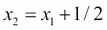
Based on the preceding equation, the correct separator will be given as:
Generating an input vector x using uniformly distributed data in R is done as follows:
#30 random numbers between -1 and 1 which are uniformly distributed
x1 <- runif(30,-1,1)
x2 <- runif(30,-1,1)
#form the input vector x
x <- cbind(x1,x2)
Now that we have the data, we need a function to classify it into one of the two categories.
#helper function to calculate distance from hyperplane
calculate_distance = function(x,w,b) {
 sum(x*w) + b
}

#linear classifier
linear_classifier = function(x,w,b) {
distances =apply(x, 1, calculate_distance, w, b)
return(ifelse(distances < 0, -1, +1))
}
The helper function, calculate_distance, calculates the distance of each point from the separator, while linear_classifier classifies each point either as belonging to class -1 or class +1.
The perceptron algorithm then uses the preceding classifier function to find the correct separator using the training data set.
#function to calculate 2nd norm
second_norm = function(x) {sqrt(sum(x * x))}

#perceptron training algorithm
perceptron = function(x, y, learning_rate=1) {

w = vector(length = ncol(x)) # initialize w
b = 0 # Initialize b
k = 0 # count iterations

#constant with value greater than distance of furthest point
R = max(apply(x, 1, second_norm))

incorrect = TRUE # flag to identify classifier

#initialize plot
plot(x,cex=0.2)

#loop till correct classifier is not found
while (incorrect ) {

 incorrect =FALSE

 #classify with current weights
 yc <- linear_classifier(x,w,b)
 #Loop over each point in the input x
 for (i in 1:nrow(x)) {
 #update weights if point not classified correctly
 if (y[i] != yc[i]) {
 w <- w + learning_rate * y[i]*x[i,]
 b <- b + learning_rate * y[i]*R^2
 k <- k+1

 #currect classifier's components
 # update plot after ever 5 iterations
 if(k%%5 == 0){
 intercept <- - b / w[[2]]
 slope <- - w[[1]] / w[[2]]
 #plot the classifier hyper plane
 abline(intercept,slope,col="red")
 #wait for user input
 cat ("Iteration # ",k,"\n")
 cat ("Press [enter] to continue")
 line <- readline()
 }
 incorrect =TRUE
 }
 }
}

s = second_norm(w)
#scale the classifier with unit vector
return(list(w=w/s,b=b/s,updates=k))
}
It's now time to train the perceptron!
#train the perceptron
p <- perceptron(x,Y)
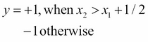
The plot will look as follows:
The perceptron working its way to find the correct classifier. The correct classifier is shown in green
The preceding plots show the perceptron's training state. Each incorrect classifier is shown with a red line. As shown, the perceptron ends after finding the correct classifier marked in green.
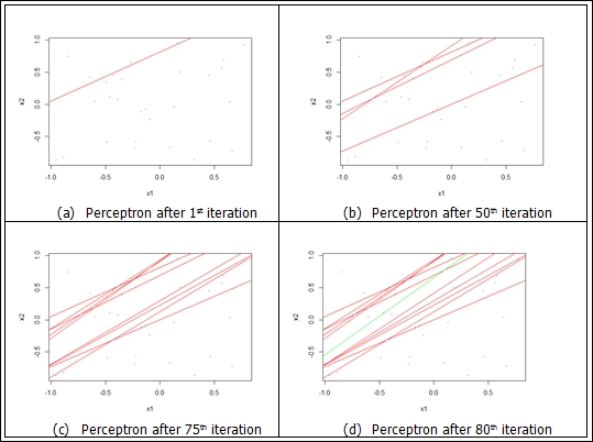
A zoomed-in view of the final separator can be seen as follows:
#classify based on calculated
y <- linear_classifier(x,p$w,p$b)


plot(x,cex=0.2)

#zoom into points near the separator and color code them
#marking data points as + which have y=1 and – for others
points(subset(x,Y==1),col="black",pch="+",cex=2)
points(subset(x,Y==-1),col="red",pch="-",cex=2)

# compute intercept on y axis of separator
# from w and b
intercept <- - p$b / p$w[[2]]

# compute slope of separator from w
slope <- - p$w[[1]] /p$ w[[2]]

# draw separating boundary
abline(intercept,slope,col="green")
The plot looks as shown in the following figure:
The correct classifier function as found by perceptron