High performance computing

Initially, it is important to measure which lines of code take the most computation time. Here, you should try to solve problems with the processing time of individual calculations by improving the computation time. This can often be done in R by vectorization, or often better by writing individual pieces of code in a compilable language, such as C, C++*, or Fortran**.

In addition, some calculations can be parallelized and accelerated through parallel computing.

Profiling to detect computationally slow functions in code

Take an example where you have written code for your data analysis but it runs (too) slow. However, it is most likely that not all your lines of code are slow and only a few lines need improvement in terms of computational time. In this instance it is very important to know exactly what step in the code takes the most computation time.

The easiest way is to find this out is to work with the R function system.time. We will compare two models:

data(Cars93, package = "MASS")
set.seed(123)
system.time(lm(Price ~ Horsepower + Weight + Type + Origin, data=Cars93))
## user system elapsed
## 0.003 0.000 0.002
library("robustbase")
system.time(lmrob(Price ~ Horsepower + Weight + Type + Origin, data=Cars93))
## user system elapsed
## 0.022 0.000 0.023

The user time is the CPU time for the call and evaluation of the code. The elapsed time is the sum of the user time and the system time. This is the most interesting number. proc.time is another simple function, often used inside functions:

ptm <- proc.time()
lmrob(Price ~ Horsepower + Weight + Type + Origin, data=Cars93)
##
## Call:
## robustbase::lmrob(formula = Price ~ Horsepower + Weight + Type + Origin, data = Cars93)
## \--> method = "MM"
## Coefficients:
## (Intercept) Horsepower Weight TypeLarge TypeMidsize
## -2.72414 0.10660 0.00141 0.18398 3.05846
## TypeSmall TypeSporty TypeVan Originnon-USA
## -1.29751 0.68596 -0.36019 1.88560
proc.time() - ptm
## user system elapsed
## 0.025 0.000 0.027

To get a more precise answer about the computational speed of the methods, we should replicate the experiment. We can see that lm is about 10 times faster than lmrob:

s1 <- system.time(replicate(100, lm(Price ~ Horsepower + Weight + Type + Origin, data=Cars93)))[3]
s2 <- system.time(replicate(100, lmrob(Price ~ Horsepower + Weight + Type + Origin, data=Cars93)))[3]
(s2 - s1)/s1
## elapsed
## 10.27

However, we don't know which part of the code makes a function slow:

Rprof("Prestige.lm.out")
invisible(replicate(100,
 lm(Price ~ Horsepower + Weight + Type + Origin, data=Cars93)))
Rprof(NULL)
summaryRprof("Prestige.lm.out")$by.self
## self.time self.pct total.time total.pct
## ".External2" 0.04 22.22 0.04 22.22
## ".External" 0.02 11.11 0.02 11.11
## "[[.data.frame" 0.02 11.11 0.02 11.11
## "[[<-.data.frame" 0.02 11.11 0.02 11.11
## "as.list" 0.02 11.11 0.02 11.11
## "lm.fit" 0.02 11.11 0.02 11.11
## "match" 0.02 11.11 0.02 11.11
## "vapply" 0.02 11.11 0.02 11.11

We can see which function calls relate to the slowest part of the code.

A more detailed output is reported by using the following. However, since the output is quite long, we have redacted it for the book version (but it is available when running the code bundle that accompanies this book):

require(profr)
## Loading required package: profr
parse_rprof("Prestige.lm.out")

Note

Plots are implemented to show the profiling results.

Further benchmarking

Finally, we will show a data manipulation example using several different packages. This should show the efficiency of data.table and dplyr.

To run the following code snippets, it is mandatory to load the following since the functionality used is included in those packages:

library(microbenchmark); library(plyr); library(dplyr);
library(data.table); library(Hmisc)

The task is to calculate the groupwise (Type, Origin) means of Horsepower, for example:

data(Cars93, package = "MASS")
Cars93 %>% group_by(Type, Origin) %>% summarise(mean = mean(Horsepower))
## Source: local data frame [11 x 3]
## Groups: Type [?]
##
## Type Origin mean
## (fctr) (fctr) (dbl)
## 1 Compact USA 117.42857
## 2 Compact non-USA 141.55556
## 3 Large USA 179.45455
## 4 Midsize USA 153.50000
## 5 Midsize non-USA 189.41667
## 6 Small USA 89.42857
## 7 Small non-USA 91.78571
## 8 Sporty USA 166.50000
## 9 Sporty non-USA 151.66667
## 10 Van USA 158.40000
## 11 Van non-USA 138.25000

First, we calculate the same with base R, where we also write a for loop for calculating the mean. We do this extra dirty for benchmarking purposes:

meanFor <- function(x){
 sum <- 0
 for(i in 1:length(x)) sum <- sum + x[i]
 sum / length(x)
}

## groupwise statistics
myfun1 <- function(x, gr1, gr2, num){
 x[,gr1] <- as.factor(x[,gr1])
 x[,gr2] <- as.factor(x[,gr2])
 l1 <- length(levels(x[,gr1]))
 l2 <- length(levels(x[,gr1]))
 gr <- numeric(l1*l2)
 c1 <- c2 <- character(l1*l2)
 ii <- jj <- 0
 for(i in levels(x[,gr1])){
 for(j in levels(x[,gr2])){
 ii <- ii + 1
 c1[ii] <- i
 c2[ii] <- j
 vec <- x[x[,gr2] == j & x[,gr1] == i, num]
 if(length(vec) > 0) gr[ii] <- meanFor(vec)
 }
 }

 df <- data.frame(cbind(c1, c2))
 df <- cbind(df, gr)
 colnames(df) <- c(gr1,gr2,paste("mean(", num, ")"))
 df
}

## groupwise using mean()
## attention mean.default is faster
myfun2 <- function(x, gr1, gr2, num){
 x[,gr1] <- as.factor(x[,gr1])
 x[,gr2] <- as.factor(x[,gr2])
 l1 <- length(levels(x[,gr1]))
 l2 <- length(levels(x[,gr1]))
 gr <- numeric(l1*l2)
 c1 <- c2 <- character(l1*l2)
 ii <- jj <- 0
 for(i in levels(x[,gr1])){
 for(j in levels(x[,gr2])){
 ii <- ii + 1
 c1[ii] <- i
 c2[ii] <- j
 gr[ii] <- mean(x[x[,gr2] == j & x[,gr1] == i, num])
 }
 }

 df <- data.frame(cbind(c1, c2))
 df <- cbind(df, gr)
 colnames(df) <- c(gr1,gr2,paste("mean(", num, ")"))
 df
}

For data.table, we will create a data table:

Cars93dt <- data.table(Cars93)

We now run the benchmark using microbenchmark and plot the results. For the plot syntax, refer to the section on visualization:

op <- microbenchmark(
 ## pure for loops
 MYFUN1 = myfun1(x=Cars93, gr1="Type", gr2="Origin",
 num="Horsepower"),
 ## pure for loops but using mean
 MYFUN2 = myfun2(x=Cars93, gr1="Type", gr2="Origin",
 num="Horsepower"),
 ## plyr
 PLYR = ddply(Cars93, .(Type, Origin), summarise,
 output = mean(Horsepower)),
 ## base R's aggregate and by
 AGGR = aggregate(Horsepower ~ Type + Origin, Cars93, mean),
 BY = by(Cars93$Horsepower,
 list(Cars93$Type,Cars93$Origin), mean),
 ## Hmisc's summarize
 SUMMARIZE = summarize(Cars93$Horsepower,
 llist(Cars93$Type,Cars93$Origin), mean),
 ## base R's tapply
 TAPPLY = tapply(Cars93$Horsepower,
 interaction(Cars93$Type, Cars93$Origin), mean),
 ## dplyr
 DPLYR = summarise(group_by(Cars93, Type, Origin),
 mean(Horsepower)),
 ## data.table
 DATATABLE = Cars93dt[, aggGroup1.2 := mean(Horsepower),
 by = list(Type, Origin)],
 times=1000L)

The output can now be visualized, see the following screenshot:

m <- reshape2::melt(op, id="expr")
ggplot(m, aes(x=expr, y=value)) +
 geom_boxplot() +
 coord_trans(y = "log10") +
 xlab(NULL) + ylab("computation time") +
 theme(axis.text.x = element_text(angle=45))

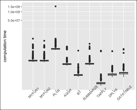
We can see that both dplyr and data.table are no faster than the others. Even the dirty for loops are almost as fast.

But we get a very different picture with large data sets:

library(laeken); data(eusilc)
eusilc <- do.call(rbind,
 list(eusilc,eusilc,eusilc,eusilc,eusilc,eusilc,eusilc))
eusilc <- do.call(rbind,
 list(eusilc,eusilc,eusilc,eusilc,eusilc,eusilc,eusilc))
dim(eusilc)
## [1] 726523 28
eusilcdt <- data.table(eusilc)
setkeyv(eusilcdt, c('hsize','db040'))

op <- microbenchmark(
 MYFUN1 = myfun1(x=eusilc, gr1="hsize", gr2="db040", 
 num="eqIncome"),
 MYFUN2 = myfun2(x=eusilc, gr1="hsize", gr2="db040", 
 num="eqIncome"),
 PLYR = ddply(eusilc, .(hsize, db040), summarise, 
 output = mean(eqIncome)),
 AGGR = aggregate(eqIncome ~ hsize + db040, eusilc, mean),
 BY = by(eusilc$eqIncome, list(eusilc$hsize,eusilc$db040), mean),
 SUMMARIZE = summarize(eusilc$eqIncome, 
 llist(eusilc$hsize,eusilc$db040), mean),
 TAPPLY = tapply(eusilc$eqIncome, 
 interaction(eusilc$hsize, eusilc$db040), mean),
 DPLYR = summarise(group_by(eusilc, hsize, db040), 
 mean(eqIncome)),
 DATATABLE = eusilcdt[, mean(eqIncome), by = .(hsize, db040)],
 times=10)

Again, we plot the results, as shown in the following screenshot:

m <- reshape2::melt(op, id="expr")
ggplot(m, aes(x=expr, y=value)) +
 geom_boxplot() + 
 coord_trans(y = "log10") +
 xlab(NULL) + ylab("computation time") +
 theme(axis.text.x = element_text(angle=45, vjust=1))

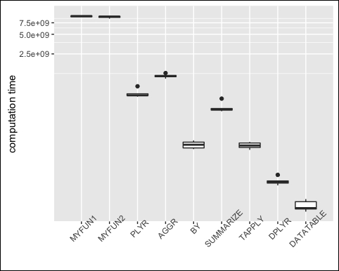
We can now observe that data.table and dylr are much faster than the other methods (the graphics shows log-scale!).

We can further profile the functions, for example, for aggregate we see that calling gsub and prettyNum needs the most computation time in function aggregate:

Rprof("aggr.out")
a <- aggregate(eqIncome ~ hsize + db040, eusilc, mean)
Rprof(NULL)
summaryRprof("aggr.out")$by.self
## self.time self.pct total.time total.pct
## "gsub" 0.52 48.15 0.68 62.96
## "prettyNum" 0.16 14.81 0.16 14.81
## "<Anonymous>" 0.10 9.26 1.08 100.00
## "na.omit.data.frame" 0.06 5.56 0.12 11.11
## "match" 0.06 5.56 0.08 7.41
## "anyDuplicated.default" 0.06 5.56 0.06 5.56
## "[.data.frame" 0.04 3.70 0.18 16.67
## "NextMethod" 0.04 3.70 0.04 3.70
## "split.default" 0.02 1.85 
 0.04 3.70
## "unique.default" 0.02 1.85 0.02 1.85

Parallel computing

Parallel computing is helpful, especially for simulation tasks, since most simulations can be done independently. Several functions and packages are available in R. For this example, we will show only a simple package, the package snow (Tierney et al., 2015). Using Linux and OS X, one can also use the package parallel, while foreach works for all platforms.

Again, the Cars93 data is used. We want to fit the correlation coefficient between Price and Horsepower using a robust method (minimum covariance determinant - MCD), and in addition we want to fit the corresponding confidence interval by a Bootstrap. For the theory of Bootstrap, refer to Chapter 3, The Discrepancy Between Pencil-Driven Theory and Data-Driven Computational Solutions. Basically, we take Bootstrap samples (using sample()) and for each Bootstrap sample we calculate the robust covariance. From the results (R values), we take certain quantiles which can then be used for determining the confidence interval:

R <- 10000
library(robustbase)
covMcd(Cars93[, c("Price", "Horsepower")], cor = TRUE)$cor[1,2]
## [1] 0.8447
## confidence interval:
n <- nrow(Cars93)
f <- function(R, ...){
 replicate(R, covMcd(Cars93[sample(1:n, replace=TRUE), 
 c("Price", "Horsepower")], cor = TRUE)$cor[1,2])
}
system.time(ci <- f(R))
## user system elapsed 
## 79.056 0.265 79.597
quantile(ci, c(0.025, 0.975))
## 2.5% 97.5%
## 0.7690 0.9504

The aim is now to parallelize this calculation. We will call the package snow and make three clusters. Note that you can make more clusters if you have more CPUs on your machine. You should use the number of CPUs you have minus one as the maximum:

library("snow")
cl <- makeCluster(3, type="SOCK")

We now need to make the package robustbase available for all nodes as well as the data and the function:

clusterEvalQ(cl, library("robustbase"))
clusterEvalQ(cl, data(Cars93, package = "MASS"))
clusterExport(cl, "f")
clusterExport(cl, "n")

We can also set a random seed for each cluster:

clusterSetupRNG(cl, seed=123)
## Loading required namespace: rlecuyer
## [1] "RNGstream"

With clusterCall we can perform parallel computing:

system.time(ci_boot <-
 clusterCall(cl, f, R = round(R / 3)))
## user system elapsed
## 0.001 0.000 38.655
quantile(unlist(ci_boot), c(0.025, 0.975))
## 2.5% 97.5%
## 0.7715 0.9512

We see that we are approximately twice as fast, and we could be even faster if we had more CPUs available.

Finally, we want to stop the cluster:

stopCluster(cl)

Interfaces to C++

Interfaces to C++ are recommended in order to make certain loops faster. We will show a very simple example to calculate the weighted mean. It should highlight the possibilities and let readers first get into touch with the package Rcpp (Eddelbuettel and Francois, 2011; Eddelbuettel, 2013), which simplifies the use of C++ code dramatically compared with R's .Call function.

Two great communicators of R, Hadley Wickham and Romain, used this example in their tutorials.

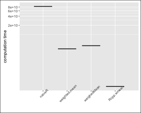
We want to compare the runtime of an example using R as an interpreted language, and also using Rcpp. We want to calculate the weighted mean of a vector.

A naive R function could look like that. We will use only interpreted R code:

wmeanR <- function(x, w) {
 total <- 0
 total_w <- 0
 for (i in seq_along(x)) {
 total <- total + x[i] * w[i]
 total_w <- total_w + w[i]
 }
 total / total_w
}

There is also a function called weighted.mean available in the base installation of R, and weightedMean in package laeken (Alfons and Templ, 2013).

Let us also define the Rcpp function. The function cppFunction compiles and links a shared library, then internally defines an R function that uses .Call:

library("Rcpp")
## from 
## http://blog.revolutionanalytics.com/2013/07/deepen-your-r-experience-with-rcpp.html 
cppFunction('
 double wmean(NumericVector x, NumericVector w) {
 int n = x.size();
 double total = 0, total_w = 0;
 for(int i = 0; i < n; ++i) {
 total += x[i] * w[i];
 total_w += w[i];
 }
 return total / total_w;
 }
')

Now, let's compare the methods:

x <- rnorm(100000000)
w <- rnorm(100000000)
library("laeken")
op <- microbenchmark(
 naiveR = wmeanR(x, w),
 weighted.mean = weighted.mean(x, w),
 weighedMean = weightedMean(x, w),
 Rcpp.wmean = wmean(x, w), 
 times = 1
)
## Warning in weightedMean(x, w): negative weights
op
## Unit: milliseconds
## expr min lq mean median uq max neval
## naiveR 92561 92561 92561 92561 92561 92561 1
## weighted.mean 5628 5628 5628 5628 5628 5628 1
## weighedMean 4007 4007 4007 4007 4007 4007 1
## Rcpp.wmean 125 125 125 125 125 125 1

Again, we draw a plot to visualize the results, as in the following screenshot globally:

m <- reshape2::melt(op, id="expr")
ggplot(m, aes(x=expr, y=value)) + geom_boxplot() + coord_trans(y = "log10") + xlab(NULL) + ylab("computation time") + the
me(
 axis.text.x = element_text(angle=45, vjust=1))