Introduction

In this chapter, we will explore the most essential question in any data visualization project: how data can be represented in both programming constructs, and its visual metaphor. Before we start on this topic, some discussion on data visualization is necessary. In order to understand what data visualization is, first we will need to understand the difference between data and information.

Data consists of raw facts. The word raw indicates that the facts have not yet been processed to reveal their meaning...Information is the result of processing raw data to reveal its meaning.

   -Rob P., S. Morris, and Coronel C. 2009

This is how data and information are traditionally defined in the digital information world. However, data visualization provides a much richer interpretation of this definition since information is no longer the mere result of processed raw facts but rather a visual metaphor of the facts. As stated by Manuel Lima, in his Information Visualization Manifesto, design in the material world, where form is regarded to follow function.

The same dataset can generate any number of visualizations, which may lay equal claim in terms of validity. In a sense, visualization is more about communicating the creator's insight into data than anything else. On a more provocative note, Card, McKinlay, and Shneiderman suggested that the practice of information visualization can be described as follows:

The use of computer-supported, interactive, visual representations of abstract data to amplify cognition.

 -"Card S. and Mackinly J.", and Shneiderman B. 1999

In the following sections, we will explore various techniques D3 provides to bridge the data with the visual domain. It is the very first step we need to take before we can create a cognition amplifier with our data.

The enter-update-exit pattern

The task of matching each datum with its visual representation, for example, drawing a single bar for every data point you have in your dataset, updating the bars when the data points change, and then eventually removing the bars when certain data points no longer exist, seems to be a complicated and tedious task. This is precisely why D3 was designed, to provide an ingenious way of simplifying the implementation of this task. This way of defining the connection between data and its visual representation is usually referred to as the enter-update-exit pattern in D3. This pattern is profoundly different from the typical imperative method most developers are familiar with. However, the understanding of this pattern is crucial to your effectiveness with the D3 library; and therefore, in this section, we will focus on explaining the concept behind this pattern. First, let's take a look at the following conceptual illustration of the two domains:

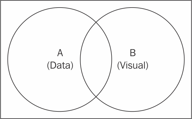
Data and visual set

In the preceding illustration, the two circles represent two joined sets. Set A depicts your dataset, whereas set B represents the visual elements. This is essentially how D3 sees the connection between your data and visual elements. You might be asking how set theory will help your data visualization effort here. Let me explain.

First, let us consider the question how can I find all visual elements that currently represent their corresponding data point? The answer is A∩B; this denotes the intersection of sets A and B, the elements that exist in both Data and Visual domains.

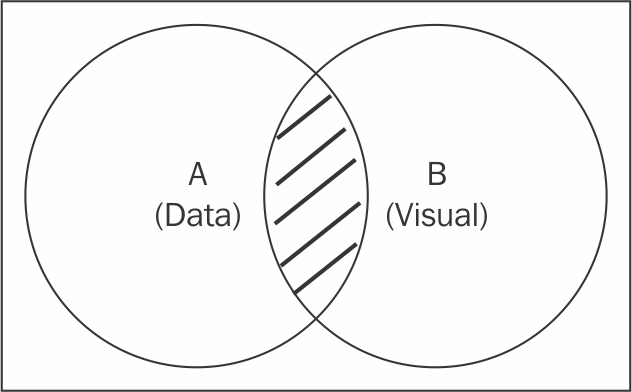
Update mode

In the preceding diagram, the shaded area represents the intersection between the two sets, A and B. In D3, the selection.data function can be used to select this intersection, A ∩ B.

The selection.data(data) function, upon selection, sets up the connection between the data domain and visual domain, as we discussed in the previous paragraph. The initial selection forms the visual set B, whereas the data provided in the data function form dataset A. The return result of this function is a new selection (a data-bound selection) of all elements existing in this intersection. Now, you can invoke the modifier function on this new selection to update all the existing elements. This mode of selection is usually referred to as the Update mode.

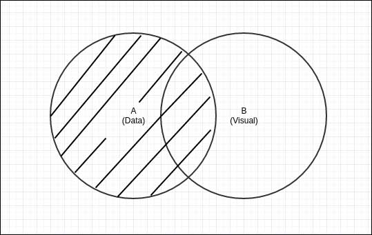
The second question we will need to answer here is how can I target data points that have not yet been visualized? The answer is the set difference of A and B, denoted as A\B, which can be seen visually through the following illustration:

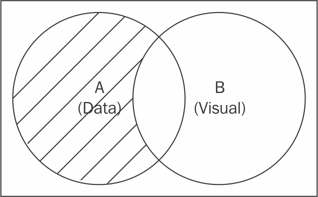
Enter mode

The shaded area in set A represents the data points that have not yet been visualized. In order to gain access to this A\B subset, the following functions need to be performed on a data-bound D3 selection (a selection returned by the data function).

The selection.data(data).enter() function returns a new selection representing the A\B subset, which contains all the pieces of data that has not yet been represented in the visual domain. The regular modifier function can then be chained to this new selection method to create new visual elements that represent the given data elements. This mode of selection is simply referred to as the Enter mode.

The third case in our discussion covers the visual elements that exist in our dataset but no longer have any corresponding data element associated with them. You might ask how this kind of visual element can exist in the first place. This is usually caused by removing the elements from the dataset; that is, if you initially visualized all data points within your dataset, and removed some data points after that. Now, you have certain visual elements that are no longer representing any valid data point in your dataset. This subset can be discovered using an inverse of the Update difference, denoted as B\A.

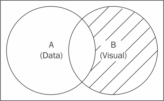
Exit mode

The shaded area in the preceding illustration represents the difference we just discussed. The subset can be selected using the selection.exit function on a data-bound selection.

The selection.data(data).exit function, when invoked on a data-bound D3 selectioncomputes a new selection which contains all visual elements that are no longer associated with any valid data element. As a valid D3 selection object, the modifier function can then be chained to this selection to update and remove these visual elements that are no longer required as part of our visualization. This mode of selection is called the Exit mode.

Together, the three different selection modes cover all possible cases of interaction between the data and its visual domain.

Additionally, D3 also offers a fourth selection mode that is very handy when you need to avoid duplicating visualization code or the so-called DRY up your code. This fourth mode is called merge mode. It can be invoked using the selection.merge function. This function merges the given selection passed to the merge function with the selection where the function is invoked and returns a new selection that is a union of both. In the enter-update-exit pattern, the merge function is commonly used to construct a selection that covers both the Enter and Update modes since that's where most code duplication would otherwise live.

Merge mode

The shaded area in this illustration shows the data points targeted by merge mode that combines both Enter and Update modes, which is essentially the entire set A. This is very convenient since now a single chain of modifiers can be utilized to style both modes and thus lead to less code duplication. We will demonstrate how to leverage merge mode in each recipe of this chapter.

Note

In software engineering, Don't Repeat Yourself (DRY) is a principle of software development, aimed at reducing repetition of information of all kinds (Wikipedia, August 2016). You can also read Mike Bostock's post on What Makes Software Good? for more insight on reasons behind this design change at https://medium.com/@mbostock/what-makes-software-good-943557f8a488#.l640c13rp .

The enter-update-exit pattern is the cornerstone of any D3-driven visualization. In the following recipes of this chapter, we will cover the topics on how these selection methods can be utilized to generate data-driven visual elements efficiently and easily.