Silhouette score

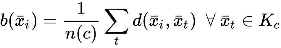
The most common method to assess the performance of a clustering algorithm without knowledge of the ground truth is the silhouette score. It provides both a per-sample index and a global graphical representation that shows the level of internal coherence and separation of the clusters. In order to compute the score, we need to introduce two auxiliary measures. The first one is the average intra-cluster distance of a sample x_i ∈ K_j assuming the cardinality of |K_j| = n(j):

For K-means, the distance is assumed to be Euclidean, but there are no specific limitations. Of course, d(?) must be the same distance function employed in the clustering procedure. 

Given a sample x_i ∈ K_j, let's denote the nearest cluster as K_c. In this way, we can also define the smallest nearest-cluster distance (as the average nearest-cluster distance):

With these two measures, we can define the silhouette score for x_i ∈ X:

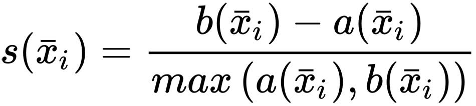
The score s(?) ∈ (-1, 1). When s(?) → -1, it means that b(?) << a(?), hence the sample x_i ∈ K_j is closer to the nearest cluster K_c than to the other samples assigned to K_j. This condition indicates a wrong assignment. Conversely, when s(?) → 1, b(?) >> a(?), so the sample x_i is much closer to its neighbors (belonging to the same cluster) than to any other point assigned to the nearest cluster. Clearly, this is an optimal condition and the reference to employ when fine-tuning an algorithm. However, as this index is not global, it's helpful to introduce silhouette plots, which show the scores achieved by each sample, grouped by cluster and sorted in descending order. 

Let's consider silhouette plots for the Breast Cancer Wisconsin dataset for K={2, 4, 6, 8} (the full code is included in the repository):

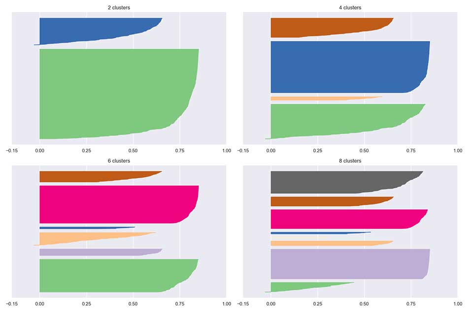
The first diagram shows the natural clustering with K=2. The first silhouette is very sharp, indicating that the average inter-cluster distance has a large variance. Moreover, one cluster has many more assignments than the other one (even if it's less sharp). From the dataset description, we know that the two classes are unbalanced (357 benign versus 212 malignant), hence the asymmetry is partially justified. However, in general, when the datasets are balanced, a good silhouette plot is characterized by homogeneous clusters with a rounded silhouette that should be close to 1.0. In fact, when the shape is similar to a long cigar, it means that the intra-cluster distances are very close to their average (high cohesion) and there's a clear separation between adjacent clusters. For K=2, we have reasonable scores, as the first cluster reaches 0.6, while the second one has a peak corresponding to about 0.8. However, while in the latter the majority of samples are characterized by s(?) > 0.75, in the former one, about half of the samples are below 0.5. This analysis shows that the larger cluster is more homogeneous and it's easier for K-means to assign the samples (that is, in terms of measures, the variance of x_i ∈ K₂ is smaller and, in the high-dimensional space, the ball representing K₂ is more uniform than the one representing K₁).

The other plots show similar scenarios because a very cohesive cluster has been detected together with some sharp ones. That means there is a very consistent width discrepancy. However, increasing K, we obtain slightly more homogeneous clusters because the number of assigned samples tends to become similar. The presence of a very rounded (almost rectangular) cluster with s(?) > 0.75 confirms that the dataset contains at least one group of very cohesive samples, whose distances with respect to any other point assigned to other clusters are quite close. We know that the malignant class (even if its cardinality is larger) is more compact, while the benign one spreads over a much wider subspace; hence, we can assume that for all K, the most rounded cluster is made up of malignant samples and all the others can be distinguished according to their sharpness. For example, for K=8, the third cluster is very likely to correspond to the central part of the second cluster in the first plot, while the smaller ones contain samples belonging to isolated regions of the benign subset. 

If we don't know the ground truth, we should consider both K=2 and K=8 (or even larger). In fact, in the first case, we are probably losing many fine-grained pieces of information, but we are determining a strong subdivision (assuming that one cluster is not extremely cohesive due to the nature of the problem). On the other side, with K>8, the clusters are obviously smaller, with a moderately higher cohesion and they represent subgroups that share some common features. As we discussed in the previous section, the final choice depends on many factors and these tools can only provide a general indication. Moreover, when the clusters are non-convex or their variance is not uniformly distributed among all features, K-means will always yield suboptimal performances because the resulting clusters will incorporate a large empty space. Without specific directions, the optimal number of clusters is associated with a plot containing homogeneous (with approximately the same width) rounded plots. If the shape remains sharp for any K value, it means that the geometry is not fully compatible with symmetric measures (for example, the clusters are very stretched) and other methods should be taken into account.