- Applied Supervised Learning with R
- Karthik Ramasubramanian Jojo Moolayil
- 436字
- 2021-06-11 13:22:31
Exploratory Data Analysis
We will get started with the dataset available to download from UCI ML Repository at https://archive.ics.uci.edu/ml/datasets/Bank%20Marketing.
Download the ZIP file and extract it to a folder in your workspace and use the file named bank-additional-full.csv. Ask the students to start a new Jupyter notebook or an IDE of their choice and load the data into memory.
Exercise 18: Studying the Data Dimensions
Let's quickly ingest the data using the simple commands we explored in the previous chapter and take a look at a few essential characteristics of the dataset.
We are exploring the length and breadth of the data, that is, the number of rows and columns, the names of each column, the data type of each column, and a high-level view of what is stored in each column.
Perform the following steps to explore the bank dataset:
- First, import all the required libraries in RStudio:
library(dplyr)
library(ggplot2)
library(repr)
library(cowplot)
- Now, use the option method to set the width and height of the plot as 12 and 4, respectively:
options(repr.plot.width=12, repr.plot.height=4)
Ensure that you download and place the bank-additional-full.csv file in the appropriate folder. You can access the file from http://bit.ly/2DR4P9I.
- Create a DataFrame object and read the CSV file using the following command:
df <- read.csv("/Chapter 2/Data/bank-additional/bank-additional-full.csv",sep=';')
- Now, use the following command to display the data from the dataset:
str(df)
The output is as follows:
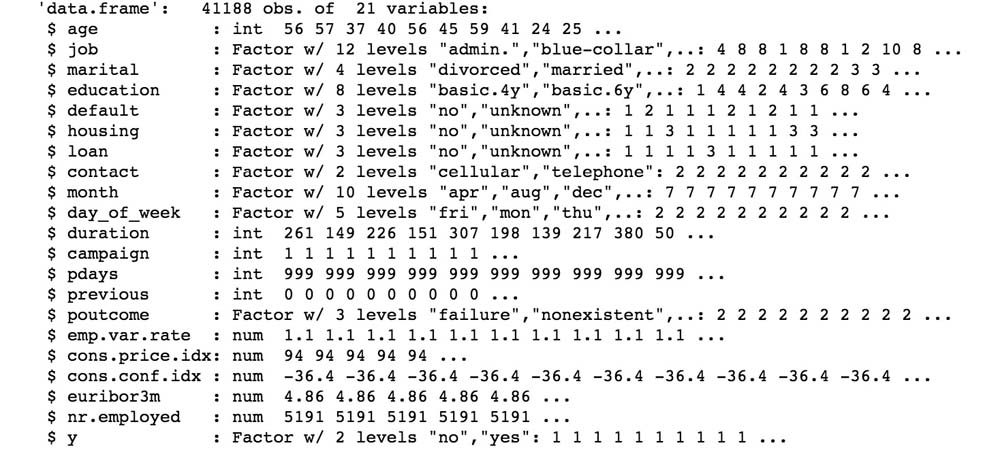
Figure 2.2: Bank data from the bank-additional-full CSV file
In the preceding example, we used the traditional read.csv function that's available in R to read the file into memory. We added an argument to the sep=";" function since the file is semicolon separated. The str function prints the high-level information we require about the dataset. If you carefully observe the output snippet, you can see that the first line denotes the shape of data, that is, the number of rows/observations and the number of columns/variables.
The next 21 lines in the output snippet give us a sneak-peek of each variable in dataset. It displays the name of the variable, its datatype, and the first few values in the dataset. We have one line for each column. The str function practically gives us a macro-view of the entire dataset.
As you can see from the dataset, we have 20 independent variables, such as age, job, and education, and one outcome/dependent variable—y. Here, the outcome variable defines whether the campaign call made to the client resulted in a successful deposit sign-up with yes or no. To understand the overall dataset, we now need to study each variable in the dataset. Let's first hop on to univariate analysis.
- Instant uTorrent
- 新型電腦主板關鍵電路維修圖冊
- Effective STL中文版:50條有效使用STL的經(jīng)驗(雙色)
- 現(xiàn)代辦公設備使用與維護
- 硬件產(chǎn)品經(jīng)理手冊:手把手構建智能硬件產(chǎn)品
- 深入淺出SSD:固態(tài)存儲核心技術、原理與實戰(zhàn)(第2版)
- 計算機組裝與維修技術
- Mastering Adobe Photoshop Elements
- Hands-On Machine Learning with C#
- CC2530單片機技術與應用
- R Deep Learning Essentials
- 微軟互聯(lián)網(wǎng)信息服務(IIS)最佳實踐 (微軟技術開發(fā)者叢書)
- Managing Data and Media in Microsoft Silverlight 4:A mashup of chapters from Packt's bestselling Silverlight books
- 可編程邏輯器件項目開發(fā)設計
- 計算機組成技術教程